Data Profiler: A tool for data drift model monitoring
Model monitoring refers to the control and evaluation of the performance of a model to determine whether or not it is operating efficiently. Machine learning typically creates static models from historical data. However, even highly accurate models are prone to decay over time once they have been deployed in production.
As demonstrated in Figure 1, the trained decision boundary (i.e. P(y|X)) is no longer valid because the input distribution of the model has changed from the initial dataset. The phenomena of data drift has been recognized as the root cause of decreased performance in many data-driven models, such as early warning systems (e.g. fraud detection) and decision support systems.
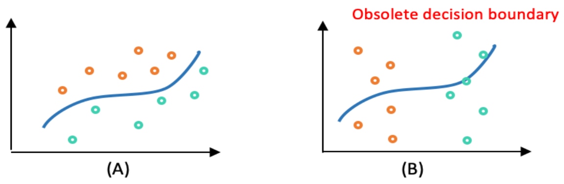
Figure 1: A) Original Data (at time t), B) Feature Drift (at time t+dt). Colors represent ground truth classes of the data points at the specified time step. The classification boundary depicted at time (t+dt) represents the previously learned relationship between features and targets at time (t).
To alleviate this problem, a framework to continuously track changes in model behavior and detect the data drift is needed.
Data drift detection framework
At the feature level, monitoring is a useful technique for identifying data drift problems. Feature drift can occur for many reasons: from data quality issues to substantive changes in the underlying data – shifts in the preferences of customers to exogenous shocks that impact behavior.
You can monitor feature drift by detecting changes in the statistical properties of each feature value over time. Some of these properties include standard deviation, average, frequency, and so on. As demonstrated in Figure 2, a general framework for data drift detection consists of the following four stages.
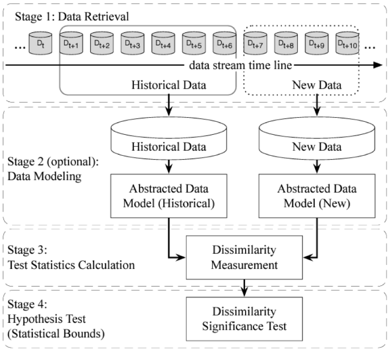
Figure 2: An overall framework for data drift detection (Image source: https://arxiv.org/pdf/2004.05785.pdf)
-
Stage 1: Data retrieval aims to retrieve data chunks from data streams.
-
Stage 2: Data modeling seeks to abstract the retrieved data and extract the key features containing sensitive information, that is, the features of the data that most impact a system if they drift.
-
Stage 3: Test statistics calculation is the measurement of dissimilarity, or distance estimation. It quantifies the severity of the drift and forms test statistics for the hypothesis test.
-
Stage 4: Hypothesis test uses a specific hypothesis test to evaluate the statistical significance of the change observed in Stage 3, or the p-value. They are used to determine drift detection accuracy by proving the statistical bounds of the test statistics proposed in Stage 3. One benefit of hypothesis testing is that it can be interpreted in terms of confidence or p-value, which shows not only how much the distributions differ but also a degree of certainty in that finding.
Kubeflow Data Profiler component
The Data Profiler is a standalone Python library built and managed by the Applied Research team at Capital One. It is designed to automate data analysis, monitoring and sensitive data detection. Data Profiler can accept a wide range of data formats including csv, avro, parquet, JSON, text, pandas DataFrames, and even point to urls of hosted data. Whether the data is structured, unstructured or graph data, the library is able to identify the schema, statistics, and entities from the data.
Adoption of Data Profiler as a Service
The entire data drift detection process (including data retrieval, data modeling, and test statistics) illustrated in Fig. 2 can be carried out with this package. We adopt Data Profiler as a Service in Kubeflow, an open-source Kubernetes-based tool for automating machine learning (ML) workflows. A distributed containerized environment like Kubernetes requires packaging ML code into containers configured with all the necessary executables, libraries, configuration files, and other data.
Model computation in a Kubernetes cluster with Kubeflow
Kubeflow pipelines is an extension of Kubeflow that allows its users to run its model computation in a controlled Kubernetes cluster. A containerized Data Profiler enables you to use this library as a component in a Kubeflow pipeline. Access to a library of reusable Kubeflow components, such as a containerized Data Profiler, provide reusable utility to library or model computations on-demand.
Pipelines can be represented as a directed acyclic graph (DAG) that are made up of one or more components. Each pipeline component is a self-contained piece of code including inputs (arguments) and outputs and performs one step in the pipeline.
For example, one component may be responsible for data preprocessing and another one for data transformation, model training, and so on. This containerized architecture solves a ubiquitous issue by making it simple to reuse, share or swap out components as workflow changes.

Figure 3: KubeflowPipeline directed acyclic graph (DAG)
Kubeflow Data Profiler components
In particular, the following operations can be included as a single task:
- ‘create_profile’: which automatically formats and loads the files, identifies the schema and gathers statistics or informative summaries of the data and It returns profile model object and corresponding report in JSON format.
- ‘update_profile’: updates the profile model object and the JSON report with the new incoming data.
- ‘merge_profiles’: allows us to retrieve data in multiple batches and profile it in a distributed manner.
- ‘diff_profiles’: takes two profiles and finds the differences b/w them and creates a difference report.
In addition, create_profile operation requires the following input parameters:
‘path_to_input_file’: which supports data in various formats such as CSV, JSON and parquet
‘path_to_output_report’: The path to the output JSON report.
‘path_to_output_profile_object’: The path to the output profile model object.
It also accepts the optional dictionary parameters including ‘read_options’, ‘report_options’ and ‘profiler_options’.
Feature drift detection using Data Profiler component
Let's say that we have a set of data that includes demographic information and credit ratings and that this data was used to train a model used to assist in loan approval decisions.
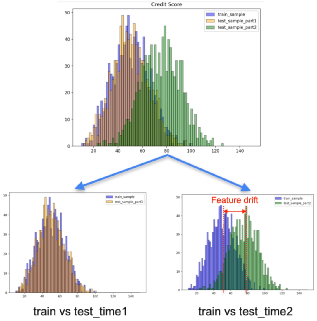
Figure 4: Distribution of credit score feature for training samples VS test (unobserved) data.
There are two batches of training samples, train_sub1, train_sub2. Additionally, two sets of new data are gathered as unobserved data over two distinct time periods, test_data_time1 and time2. Given the distribution of credit score for different samples, figure 4, We anticipate to detect a feature drift between training samples and test data time2.
We created a feature drift detection pipeline using a containerized Data Profiler component. Figure 5 demonstrates an overview of the Kubeflow Data Profiler pipeline used to detect feature drift. The containerized architecture makes it simple to reuse Data Profiler components with varied operations as needed by workflow. After running the pipeline, you are able to explore the results on the pipeline interfaces, debug, tweak parameters, and run experiments by executing the pipeline with different parameters or data sources.
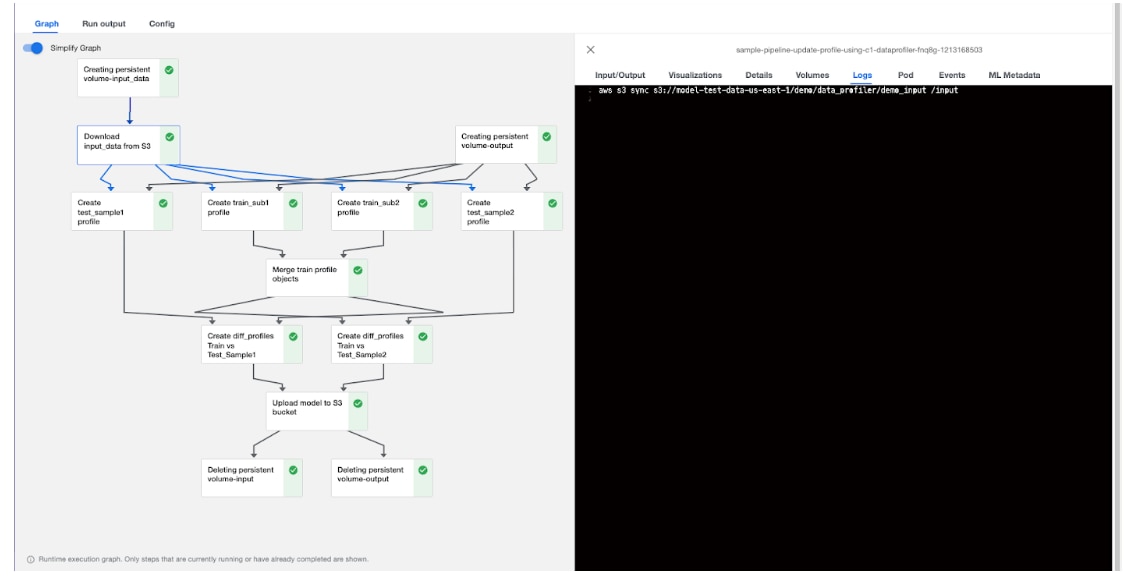
Figure 5: An overview of Kubeflow DataProfiler pipeline ran for feature drift detection - observing logs from pipeline run.
Initial steps included creating a persistent volume and downloading data samples to a common input persistent volume (PV). A persistent volume is a storage component utilized by a Kubernetes cluster whose lifecycle is independent of any containers, pods and nodes that use the PV. Multiple pods can read and write to the same shared PVs simultaneously. They are defined by an API object, which captures the implementation details of storage such as NFS file shares, or specific cloud storage systems, shown below.
    # Create Shared Volumes
vol_resource_name = f"data-vol-{int(time.time())}"
dir_vol_data = (
    kfp.dsl.VolumeOp(
        name=vol_resource_name,
        resource_name=vol_resource_name,
        storage_class="managed-nfs-storage",
        size="10M",
        modes=kfp.dsl.VOLUME_MODE_RWM,
    )
    .add_pod_annotation(
        name="pipelines.kubeflow.org/max_cache_staleness", value="P0D"
    )
    .set_display_name("Creating persistent volume-input_data")
)
vol_resource_name = f"output-vol-{int(time.time())}"
dir_vol_output = (
    kfp.dsl.VolumeOp(
        name=vol_resource_name,
        resource_name=vol_resource_name,
        storage_class="managed-nfs-storage",
        size="5M",
        modes=kfp.dsl.VOLUME_MODE_RWM,
    )
    .add_pod_annotation(
        name="pipelines.kubeflow.org/max_cache_staleness", value="P0D"
    )
    .set_display_name("Creating persistent volume-output")
)
Next, profiles for train sample sub1 and sub2 and test samples each were created using separate create_profile operators in a distributed manner.
    path_to_input_file = os.path.join(str(local_path_to_input_folder), "train_sub1.csv")

create_profile_op1 = profiler_component(
   method_name="create_profile",
   kwargs={
       "path_to_input_file": path_to_input_file,
       "read_options": read_options,
       "report_options": report_options,
       "profiler_options": profiler_options,
       "path_to_output_report": "/output/report_train_sub1.json",
       "path_to_output_profile_object": "/output/train_sub1_profile.pkl",
   },
)

create_profile_op1 = resources.node_selector(create_profile_op1, size="micro")
create_profile_op1.set_display_name("Create train_sub1 profile")
create_profile_op1.add_pvolumes({local_path_to_input_folder: dir_vol_data.volume})
create_profile_op1.add_pvolumes(
   {local_path_to_output_folder: dir_vol_output.volume}
)
create_profile_op1.execution_options.caching_strategy.max_cache_staleness = "P0D"
create_profile_op1.after(s3_download_op)
The following stage, shown in the below code snippet and Figure 6, involved merging train profile objects using the merge_profile operator.
    merge_profiles_op = profiler_component(
       method_name="merge_profiles",
       kwargs={
           "path_to_input_profile_objects": "['/output/train_sub1_profile.pkl', '/output/train_sub2_profile.pkl']",
           "report_options": report_options,
           "path_to_output_report": "/output/report_train_merged.json",
           "path_to_merged_profile_object": "/output/train_merged_profile.pkl",
       },
   )


merge_profiles_op = resources.node_selector(merge_profiles_op, size="micro")
merge_profiles_op.set_display_name("Merge train profile objects")
merge_profiles_op.add_env_variable(env_var)
merge_profiles_op.add_pvolumes({local_path_to_input_folder: dir_vol_data.volume})
merge_profiles_op.add_pvolumes({local_path_to_output_folder: dir_vol_output.volume})
merge_profiles_op.execution_options.caching_strategy.max_cache_staleness = "P0D"
merge_profiles_op.after(create_profile_op1).after(create_profile_op2)

Figure 6: An overview of Kubeflow DataProfiler pipeline ran for feature drift detection - observing log window for the ”merge train profile objects” component.
The diff_profile components generate the difference reports by comparing the profile of the training sample with respect to the test samples part1 and part2, respectively. The component compares the test statistics, measures drift and returns the difference report.
Data drift evaluation
One of the first and most fundamental steps that must be conducted to evaluate data drift between samples is to calculate the difference between descriptive statistics. These metrics include measures of data quality (data type, order), measures of central tendency (mean, median, mode), measures of variability (min/max, sum, variance, standard deviation), and measures of frequency (sample size, null count, and null-sample size ratio).
In addition, hypothesis testing such as t-test (in case of normally distributed features) and Population Stability Index (PSI) can be used to provide a rigorous and automatable way of comparing feature distributions. The data drift is determined to be statistically significant (p-value<1.0e-3) using the t-test for the feature of credit score between train sample and test sample part 2, as expected and depicted in Figure 7.
At the end, the results include profile model objects and JSON reports uploaded to the local directory or cloud storage such as S3 bucket and deleted persistent volumes.
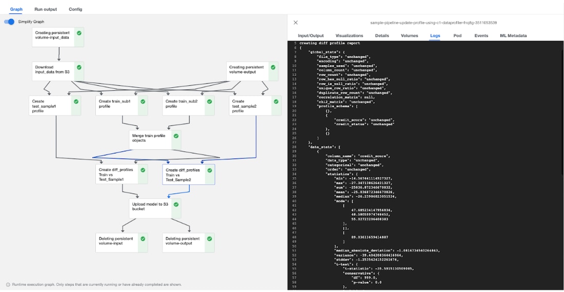
Figure 7: Kubeflow DataProfiler pipeline ran for feature drift detection - observing log window for the Create diff_profiles Train vs Test_sample2 component. Descriptive statistics drift has been reported in key-value pairs. Also, Test statistics p_value <=1.0 e-3 rejects the Null Hypothesis representing detection of data drift for credit score feature.
Data drift model monitoring tool by Capital One: In summary
In summary, we developed a data drift model monitoring tool using a containerized Data Profiler component within Kubeflow pipeline on Kubernetes cluster. The Data Profiler is a Python library designed to make data analysis, monitoring, and sensitive data detection easy. The pipeline consists of multiple components, each of which performs a single pipeline workflow task, including
- Retrieving batches of training and test samples in a distributed manner
- Profiling the data
- Merging the profile model objects
- Computing the dissimilarity metrics between distributions of data using various statistical measurements (deterministic and probabilistic).
A difference report that contains key-value pairs for several data drift measures is eventually returned by the pipeline.
Thank you for the contributions from my colleagues Jeremy Goodsitt, Sr. Mgr, Machine Learning Engineering, Applied Research, and Taylor Turner, Lead Machine Learning Engineer, Applied Research.