Gradient boosting: Tips to control your XGBoost model

Updated July 20, 2023

Gradient boosting is a popular machine learning technique used throughout many industries because of its performance on many classes of problems. In gradient boosting small models—called “weak learners” because individually they do not fit well—are fit sequentially to residuals of the previous models. These weak models perform with excellent predictive accuracy when added together into an ensemble. This performance comes at the cost of high model complexity which makes them hard to analyze and can lead to overfitting.

As a data scientist in the Model Risk Office, it is my job to make sure that models are fit appropriately and are analyzed for weaknesses.

1. Make each learner in the ensemble weaker.
2. Have fewer learners in the ensemble.

One of the most popular boosting algorithms is the gradient boosting machine (GBM) package XGBoost. XGBoost is a lighting-fast open-source package with bindings in R, Python, and other languages. Due to its popularity, there is no shortage of articles out there on how to use XGBoost. Even so, most articles only give broad overviews of how the code works. 

In this deep dive into XGBoost I want to discuss what I see as a common misconception about XGBoost - that the complexity of each learner and the number of learners are just two sides of the same coin. I will discuss how these two methods of controlling complexity are not the same: depth adds interactions and grows complexity faster than adding trees.

XGBoost has a few different modes, but the one I will focus on here uses tree models as the individual learners in the ensemble. The XGBoost documentation contains a great introduction which I will summarize below.

Start with some target—either continuous or binary—and some base level predictions (usually either 0 or probability of 0.5). The basic idea is to build a tree that predicts the residuals between our base predictions and the target. At each stage, we recompute the residuals and then build a new tree. We add this tree to the mode, recompute the residuals again, and repeat this process until we have a model that fits well.

The trees are built using binary splits—these are just threshold cuts in single features (unlike H2O and some other packages, XGBoost handles only continuous data—even categorical features are treated as continuous). Here would be an English-language example of a split: all customers with an account balance <$1000 go right and all customers with an account balance >=$1000 go left. 

How to pick the place to split? XGBoost looks at which feature and split-point maximizes the gain. The maximum gain is found where the sum of the loss from the child nodes most reduces the loss in the parent node. In math this is given by:

The G terms give the sum of the gradient of the loss function and the H terms give the sum of the Hessian (XGBoost just uses the second partial derivative) of the loss function. G_L is the sum of the gradient over the data going into the left child node, and G_R is the sum of the gradient over the data going into the right child node; similarly for H_L and H_R. Alpha and Lambda are the L1 and L2 regularization terms, respectively. The gain is a bit different for each loss function. See the appendix below for the two most common ones.

For small datasets, XGBoost tries all split points (thresholds) given by the data values for each feature and records their gain. It then picks the feature and threshold combination with the largest gain.

For larger datasets (by default any dataset with more than 4194303 rows), XGBoost proposes fewer candidate splits. The locations of these candidate splits are decided by the quantiles of the data (weighted by the Hessian).

During the tree building process, XGBoost automatically stops if there is a node without enough cover (the sum of the Hessians of all the data falling into that node) or if it reaches the maximum depth.

After the trees are built, XGBoost does an optional 'pruning' step that, starting from the bottom (where the leaves are) and working its way up to the root node, looks to see if the gain falls below gamma (a tuning parameter—see below). If the first node encountered has a gain value lower than gamma, then the node is pruned and the pruner moves up the tree to the next node. If, however, the node has gain higher than gamma, the node is left and the pruner does not check the parent nodes.

Now that we have the basics, let's look at the ways a model builder can control overfitting in XGBoost.

The four methods to control overfitting

There are many ways of controlling overfitting, but they can mostly be summed up in four categories:

• Regularization
• Pruning
• Sampling
• Early stopping

The regularization parameters act directly on the weights:

• lambda - L2 regularization. This term is a constant that is added to the second derivative (Hessian) of the loss function during gain and weight (prediction) calculations. This parameter can both shift which splits are taken and shrink the weights.
• alpha - L1 regularization. This term is subtracted from the gradient of the loss function during the gain and weight calculations. Like the L2 regularization it affects the choice of split points as well as the weight size.

• eta (learning_rate) - Multiply the tree values by a number (less than one) to make the model fit slower and prevent overfitting.
• max_delta_step - The maximum step size that a leaf node can take. In practice, this means that leaf values can be no larger than max_delta_step * eta.

Pruning removes splits directly from the trees during or after the build process (see more below):

• gamma (min_split_loss) - A fixed threshold of gain improvement to keep a split. Used during the pruning step of XGBoost.
• min_child_weight - Minimum sum of Hessians (second derivatives) needed to keep a child node during partitioning. Making this larger makes the algorithm more conservative (although this scales with data size). Since the second derivatives are different in classification and regression, this parameter acts differently for the two contexts. In regression this is just floor on the number of data instances (rows) that a node needs to see. For classification this gives the required sum of p*(1-p), where p is the probability, for data that are split into that node. Since probability ranges from 0 to 1, p*(1-p) ranges from 0 to 0.25 and so you will need at least four times the min_child_weight rows in that node to keep it
• max_depth - The maximum depth of a tree. While not technically pruning, this parameter acts as a hard stop on the tree build process. Shallower trees are weaker learners and are less prone to overfit (but can also not capture interactions - see below).

Sampling makes the boosted trees less correlated and prevents some feature masking effects. This makes them less correlated and more robust to noise:

• subsample - Subsample rows of the training data prior to fitting a new estimator.
• colsample_*(bytree, bylevel, bynode) - Fraction of features to subsample at different locations in the tree building process.

Early stopping monitors a metric on a holdout dataset and stops building the ensemble when that metric no longer improves:

• The XGBoost documentation details early stopping in Python. Note: this parameter is different than all the rest in that it is set during the training not during the model initialization. Early stopping is usually preferable to choosing the number of estimators during grid search.

Larger, more complex, models can be prone to overfitting, slower to score, and harder to interpret. For those reasons, knowing just how complex your model is can be beneficial. Once you've built a model using one of the above parameters, how can you figure out how complex it is? How can you compare the complexity of two different models? 

Typically, modelers only look at the parameters set during training. However, the structure of XGBoost models makes it difficult to really understand the results of the parameters. One way to understand the total complexity is to count the total number of internal nodes (splits). We can count up the number of splits using the XGBoost text dump:

There are two basic ways in which tree ensemble models can be complex:

1. Deeper trees (each estimator is more complicated)
2. More trees

These two types of complexity are not simply two sides of the same coin. They give different behaviors to the ensemble. But let's first look at just the number of nodes. 

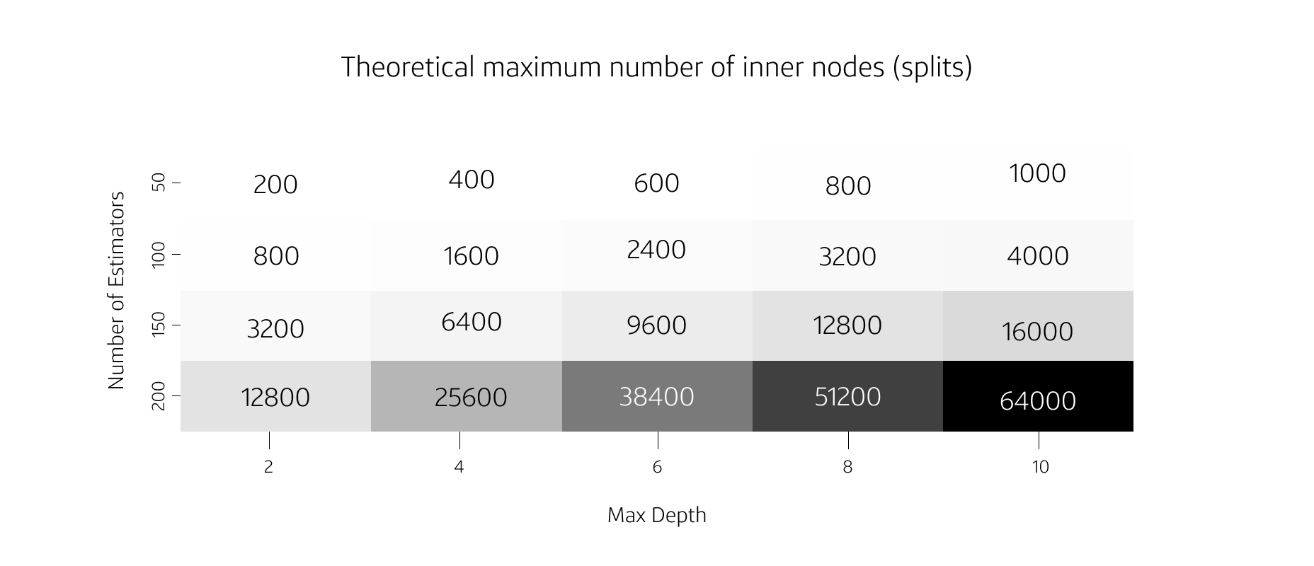
The theoretical maximum number of nodes is: n_estimators*2**max_depth . For a grid of different max_depth and n_estimator values we can see what these theoretical maximums are:

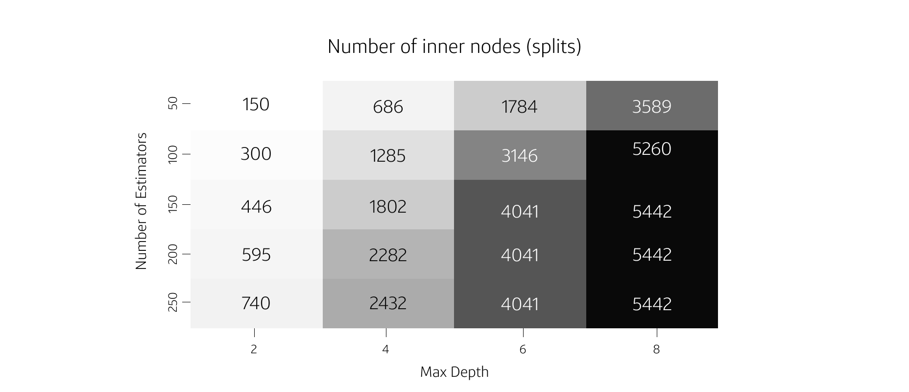
In practice, model builders should be using early stopping and pruning so the real numbers would be lower. To demonstrate, let's first look at the total complexity (number of splits) that arises from making ensembles with different max_depth and n_estimators. Note that each of these models is made with early stopping and pruning.

In practice, deeper trees tend to be more complex than shallower trees, even when we use more estimators.

Below are two of these models within  0.02 AUROC of each other. Each model was built on the classic UCI ‘adult’ machine learning problem (where we try to predict high earners). We can see the difference in how their complexity is reached. The shallower trees have many fewer leaves (end nodes - and a similarly small number of split). The deeper trees have more nodes. Both models use early stopping and so the model built with deeper trees stops building first, and yet still manages to have about 1000 extra nodes compared to the shallower ensemble.

Although every situation is different, deeper trees tend to add complexity in the form of extra leaves faster than shallower trees. This is true even though ensembles built with deeper trees tend to have fewer trees.

But complexity is not usually what model builders care about. What about the holdout AUROC for these models? In the figure below we see the results for many different models built on the same dataset, but with different tuning parameters. We can see that as complexity increases (counted by the total number of splits in the ensemble) the model performance increases up to around 1500 total splits. After that the complexity increases while the performance stays largely flat.

Extra complexity can help fit better models, but often gives diminishing returns to hold-out performance.

Complexity is not the only reason to be wary of making your trees deeper. Deeper trees add interactions in a way that adding more trees does not. Adding depth adds complexity in two ways:

1. Allows the possibility for more complicated interactions
2. Additional splits (more granular space partition)

Adding trees only adds to the second complexity. Interactions between features require a depth of trees that is deep enough to handle the interaction. Simply adding more trees will not increase the complexity of the interactions. That is, if you have a maximum depth of two, then at most two variables can interact together. I will demonstrate this using my favorite toy example: a model with four features, two of which interact strongly in an 'x’-shaped function (y ~ x1 + 5x2 - 10x2*(x3 > 0)).

Building a modest number (200) of depth-two trees will capture this interaction right away as you can see in the individual conditional expression (ICE) plot below:

If you haven’t seen ICE plots before, they show the overall average model prediction (the red line) and the predictions for a sample of data with different configurations of input features (the black lines). The model is picking up on the strong ‘x’ shape.

Modeling the same data using single split trees will never capture the interaction. Even after adding 1000 trees, the model still only shows the average effects (which is mostly flat except for some effects at the tails):

The fact that all the black lines follow the same trend shows that there is no interaction in this model.

Depth is sometimes necessary to capture interactions between features.

A corollary to this is that if there are no interactions in the dataset, then there is no need for deep trees.

While adding trees cannot add interaction complexity, it can help approximate the functional forms of the features. In these two examples we have univariate functions: sin(x) and x^2. Adding additional depth one trees can approximate these functions well, but notice that it takes many of these small trees to approximate smooth shapes:

Just as you should be automatically controlling the size of the ensemble by using early stopping, you can control the size of each individual tree using pruning. XGBoost has two basic ways of automatically controlling the complexity of the trees: gamma and min_child_weight.

Of these, only gamma is used for "pruning." Splits that have a gain value less than gamma are pruned after the trees are built. gamma is compared directly to the gain value of the nodes and therefore has to be tuned based on your particular problem.

There is a nuance about pruning in XGBoost. If you look at the distribution of the gains in your model, you might see something like this:

The vertical line shows gamma and the blue histogram shows the number of splits (nodes) at different values of gain. Why do some splits survive even with less gain than gamma? The reason is that the XGBoost pruning happens from the bottom up. If XGBoost does not prune a node because it has higher gain than gamma, then it will not check any of the parent nodes. This means that splits can have low gain and still survive as long as their descendants have high enough gain.

The other complexity parameter, min_child_weight, is used at build time. Any node that has a smaller cover than min_child_weight has its gain set to 0, and the tree building process along that branch stops.

The cover for a particular node is computed as the sum of the second derivatives of the loss function over all the training data falling into that node. For an XGBoost regression model, the second derivative of the loss function is 1, so the cover is just the number of training instances seen. For classification models, the second derivative is more complicated: p * (1 - p), where p is the probability of that instance being the primary class.

Because min_child_weight cares about the sum of this quantity, it will have different behavior depending on what probability the model is predicting.

XGBoost and other gradient boosting tools are powerful machine learning models that have become incredibly popular across a wide range of data science problems. 

Because these methods are more complicated than other classical techniques and often have many different parameters to control it is more important than ever to really understand how the model works. While this is especially important in highly regulated industries like banking, it is important for data scientists everywhere.

Pruning, regularization, and early stopping are all important tools that control the complexity of XGBoost models, but they come with many quirks that can lead to unintuitive behavior. By learning more about what each parameter in XGBoost does you can build models that are smaller and less prone to overfit the data.

***

Wood photo created by ingram from www.freepik.com